MS Excel, Conditional Formatting, Icon Sets
SolvedSonyXperiaSP Posted messages 134 Registration date Status Membre Last intervention -
Hello everyone,
I created a workbook with MS Excel 2024. It is used to track my cellar stock to avoid running out of something, or conversely, overstocking when there are no promotions.
Online, I listed each item.
In columns, I have the quantities every 15 days.
I need help creating conditional formatting.
I want Excel to compare the values of the cells row by row and assign a "triangle icon": a green triangle when it increases, an orange bar when it's stable, and a red triangle when it decreases.
So Excel should compare M & N and put the icon in N, N & O and place the icon in O, and so on.
For example, Excel will place a horizontal bar in cells M701 to O701, a green triangle in P701, and a horizontal bar in Q701.
How should I set the rules please?
Thank you for your patience and help;
3 réponses
In the end, I cheated a bit by tinkering.
It's not exactly what I wanted, but I'll manage on my own:
1) I created a sheet BaseFormule! which is a copy of the sheet Base!

To avoid errors, I only kept the column titles from Base! and from cell A2 of the BaseFormule! sheet, I put =Base!A2
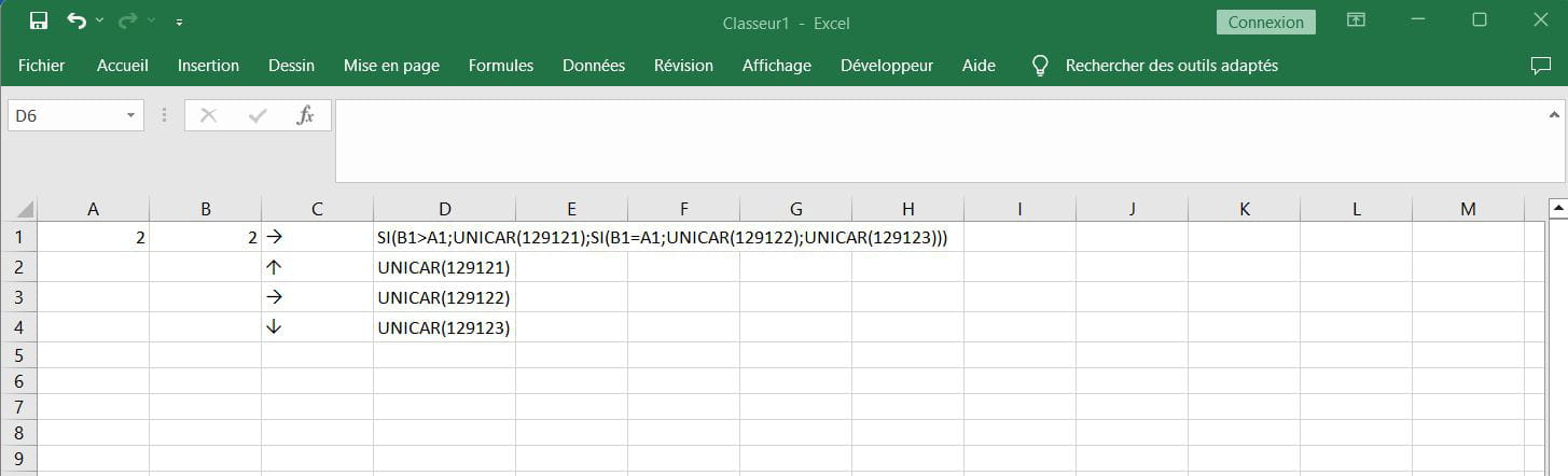
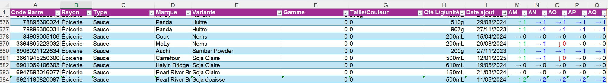
2) Knowing that my numeric data starts in Base!M2 and that the comparison should start at Base!L2, I put the following formula in BaseFormule!L2:
=IF(Base!L2<base base="" if="" />Base!M2; "↓ " & Base!M2; "→ " & Base!M2))
If M2<l2: followed="" by="" the="" value="" of="" l2="" /> If M2>L2: ↓ followed by the value of L2
If M2=L2: → followed by the value of L2
3) I dragged the formula through all the rows of the column, then through all the columns.
4) then I made 4 conditional formatting.
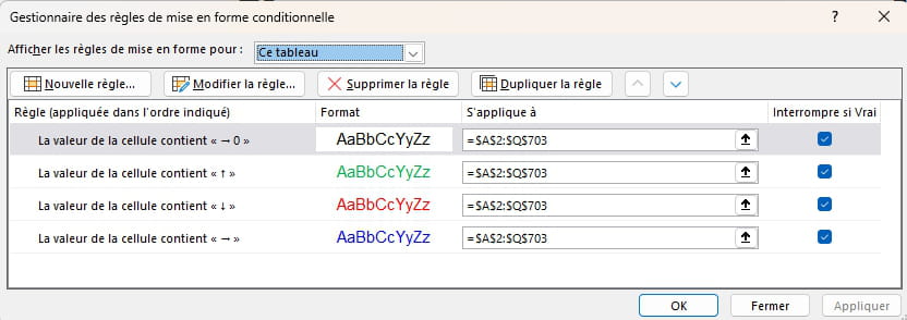
In the end, it looks pretty good for a homemade spreadsheet. :-)
Hello,
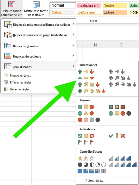
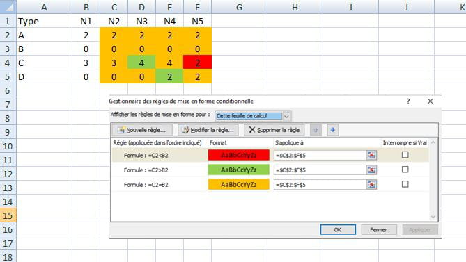
Icon sets only compare values, not cell references.
You can display the trend as follows, but with only one icon set (zero progression will be a horizontal bar).
https://planete-excel.fr/afficher-une-tendance-avec-un-jeu-dicones/

Hello
Is it possible to not use the icon set but simply color the table cells orange if the value is equal to the previous cell, green if the value is greater than the previous cell, and red for a lower value?
Best regards
Via
Hello,
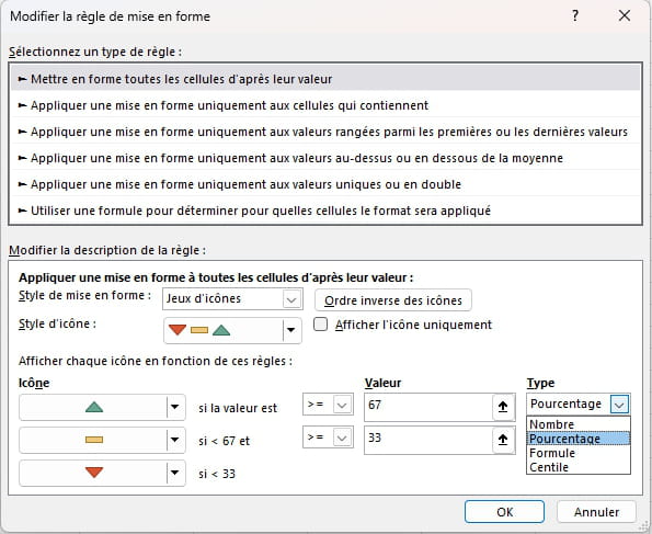
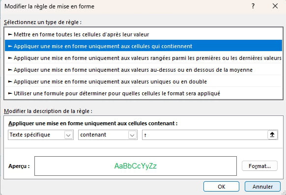
There is nothing preventing the use of a non-colored (gray) icon set, which contradicts the initial request and the reservations I highlighted in the link in <1> regarding the use of icon sets (an artifice is needed for the comparison value to be numerical).
Conditional formatting in this format relies on colors; otherwise, it has no interest, although different filling textures of the same color can be used, but it is not very readable.
If one insists on their arrows and they are not colored, one can add a cell for each comparison and use a font that supports the corresponding Unicode, for example, Segoe UI Symbol.