Single Column Occurrence Chart
Solved
Shadow
-
Shadow -
Shadow -
Hello everyone,
I'm sorry if the question has already been asked but I'm really struggling with it.
I would like to create a chart from a column to retrieve values and display them.
Example:
Column A:
Amount
€0.88
€2.06
€1.50
€1.50
€1.52
€1.40
€0.00
€2.06
€1.48
€1.61
€1.00
€1.50
€2.00
€2.10
€5.00
€2.30
€1.40
I want my chart to display each identical value once, and calculate the number of occurrences as well as the percentage.
When I do it, it only shows 1,2,3,4,5... I don't have the occurrences or the desired values.
I don’t understand, can you please help me?
I'm sorry if the question has already been asked but I'm really struggling with it.
I would like to create a chart from a column to retrieve values and display them.
Example:
Column A:
Amount
€0.88
€2.06
€1.50
€1.50
€1.52
€1.40
€0.00
€2.06
€1.48
€1.61
€1.00
€1.50
€2.00
€2.10
€5.00
€2.30
€1.40
I want my chart to display each identical value once, and calculate the number of occurrences as well as the percentage.
When I do it, it only shows 1,2,3,4,5... I don't have the occurrences or the desired values.
I don’t understand, can you please help me?
5 answers
-
Fortunately, Excel offers a remarkable tool, the Pivot Table!
- Click in A1
- Select INSERT/Pivot Chart and click OK without making any changes in the window
- In the VALUES area, at the bottom right, click on the arrow of the field "Sum of Amount", then on "Value Field Settings" and select Count instead of Sum
- Drag the field "Amount" to the top of the pane, and drop it into the AXIS (CATEGORIES) area
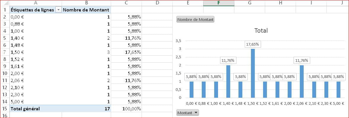
A table has been created with columns A and B, and a chart occupying the range E2:I16 ...

Right-click on one of the blue bars and click on "Add Data Labels";
you will see 1, 2, or 3 appear, the number of occurrences.
https://www.cjoint.com/c/JBvbSQddkto
--
Retirement is great! Especially in the Caribbean...
Raymond (INSA, AFPA) -
Thank you Raymond,
It took me a while to understand what you meant, but in the end, it's perfect, it's exactly what I wanted...
Indeed, in my tests I was really very, very far from this approach.
A big thank you. -
Hello.
You had expressed the wish to display the percentages... Indeed, showing the number of occurrences doesn't add much, since the graduated vertical axis immediately provides the information.- In C2, enter the formula =B2/B$15 and copy it down to C15; set the cell format to Number / Percentage

- Right-click on one of the labels, then select "Format Data Labels"; check Value from Cells ; uncheck Value ; select C2:C14 with the mouse: the small window will display =Shadow!$C$2:$C$14
- You can remove the "Total" legend on the right.
https://www.cjoint.com/c/JBwn2OjLy5o
--
Retirement is great! Especially in the Caribbean...
Raymond (INSA, AFPA) - In C2, enter the formula =B2/B$15 and copy it down to C15; set the cell format to Number / Percentage
-
It's all good once I got the expected result, I looked around a bit to see how it worked, and I found the %
Thanks again for the quick response -
Good evening.
You're not getting it because you don't understand how a chart works:
It doesn't do any calculations, statistics, or analyses.
You need to do that work in your table.
In fact, the chart merely translates the values grouped by columns in a table into a visual format. But a single column is not a table!
--
Retirement is great! Especially in the West Indies...
Raymond (INSA, AFPA)