Formatting Sheet and Adding Color
Solved
angelinas32
Posted messages
16
Status
Member
-
angelinas32 -
angelinas32 -
Hello,
I need help with conditional formatting in Sheets.
I have no problem in Excel, but in Sheets, I can't find how to do it. Could you help me?
I need to enter phone numbers in my column B, but if I write the same number, I want it to appear in a different color, like green, so I know that I have already communicated with that number during the day.
Thank you for your help.
I need help with conditional formatting in Sheets.
I have no problem in Excel, but in Sheets, I can't find how to do it. Could you help me?
I need to enter phone numbers in my column B, but if I write the same number, I want it to appear in a different color, like green, so I know that I have already communicated with that number during the day.
Thank you for your help.
Related links:
- Sheets: Color a cell with multiple colors based on different conditions
- Conditional formatting for deadlines Google Sheets
- Google Sheets: Format a row based on whether the date is past or not.
- Google Sheets: Conditional Formatting for Expired Dates.
- Google Sheets formatting during Google Forms increment.
- Cascade List Google Sheets
4 answers
-
Hello,
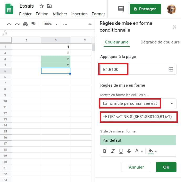
After selecting the range to process (e.g. A1:A100); tab "Format"; click on "Conditional Formatting" which opens a window on the right side of the screen
under "Format cells if" expand the dropdown list and go to the bottom and click on "Custom formula is"; enter the formula below; choose the color.
=AND(A1<>"",COUNTIF($A$1:$A$100,A1)>1)
This formula will color all filled cells whose value appears at least twice.
Best regards-
Hello
It doesn't work.
Let me explain, in my column b I write the phone numbers received during the day in order to return calls.
To avoid calling the same person multiple times, I want that if I write a number, for example in line 52, but it has already been written in line 30, both numbers should be colored so that I can delete one to avoid calling again.
Unfortunately, the function I created doesn't color my numbers even though I've selected the color.
My numbers are formatted as (000) 000-0000
Thank you
-
-
Re
In the given formula, have you corrected the letter, that is B instead of A - see my example below, if it starts on line 2 also modify the starting number - also modify the end number if the range ends before or after the one I wrote
And also be careful to write the phone numbers in the same way so that the MFC works, no spaces before or after, etc....

Best regards-
Hello,
I already have a conditional formatting set up so that when I enter the numbers, they appear as (000) 000-0000
My numbers start from row C3 and end at row C500.
I wrote this =AND(C1<>"";COUNTIF($C$3:$C$500;C3)>1) and in the formatting style I set the color to yellow but still the duplicate numbers do not turn yellow. Can you please clarify, maybe I’m doing something wrong.
THANK YOU :)
-
-
To improve things, the reference of the first C needs to change
=AND(C3<>"";COUNTIF($C$3:$C$500;C3)>1)
C3<>"" to indicate that the coloring should not be applied to empty cells in the range to be processed
Best regards-
-
This means that I am asking at the same time (hence the use of AND)
That the cells are filled (C3<>"") If we don't include this, all the empty cells in the area will be colored if there are two or more of them.
That there is the presence of a number at least twice (NB.SI($C$3:$C$500;C3)>1)
In summary, if you have selected the range C3 to C500 and you have entered the formula
=AND(C3<>"";NB.SI($C$3:$C$500;C3)>1) in the conditional formatting, everything should work
Best regards -
Hello,
Unfortunately, the numbers that turn yellow in my file are only listed once in my table. Is that normal? Why is it that only one of the two identical numbers in my table turns yellow and not both? Is there a problem?
Thank you -
Hello,
It's not working, I write in my cells C4, C5, C6, and C7 (000) 000-1111 (to do my test) and it’s cell C3 that turns yellow, but in cell C3 is today’s date. My formula is this: =AND(C4<>"",COUNTIF($C$4:$C$500,C4)>1). I would like cells C4, C5, C6, and C7 to be yellow if they contain the same number.
Thank you for your help. -
-
-