Google Sheets: Format a row based on whether the date is past or not.
papaouin
Posted messages
3
Status
Member
-
PapyLuc51 Posted messages 4567 Registration date Status Member Last intervention -
PapyLuc51 Posted messages 4567 Registration date Status Member Last intervention -
Hello,
I want to set up an action plan for ongoing/completed tasks in my company.
To facilitate reading, I would like the entire line to turn gray once the task is finished (Example: Action completed on 10/03/2020 while we are on 11/03/2020).
However, after trying several times I am encountering several problems:
1. The formatting does not apply to all formulas.
2. The formula does not adapt to the chosen cell if I drag it down.
3. When I insert a row below, the entire format of the row does not replicate. Do you have a trick?
The purpose of this document is to hand it over to my salespeople so they can fill it out as easily as possible. Therefore, everything should be optimized when they add a row.
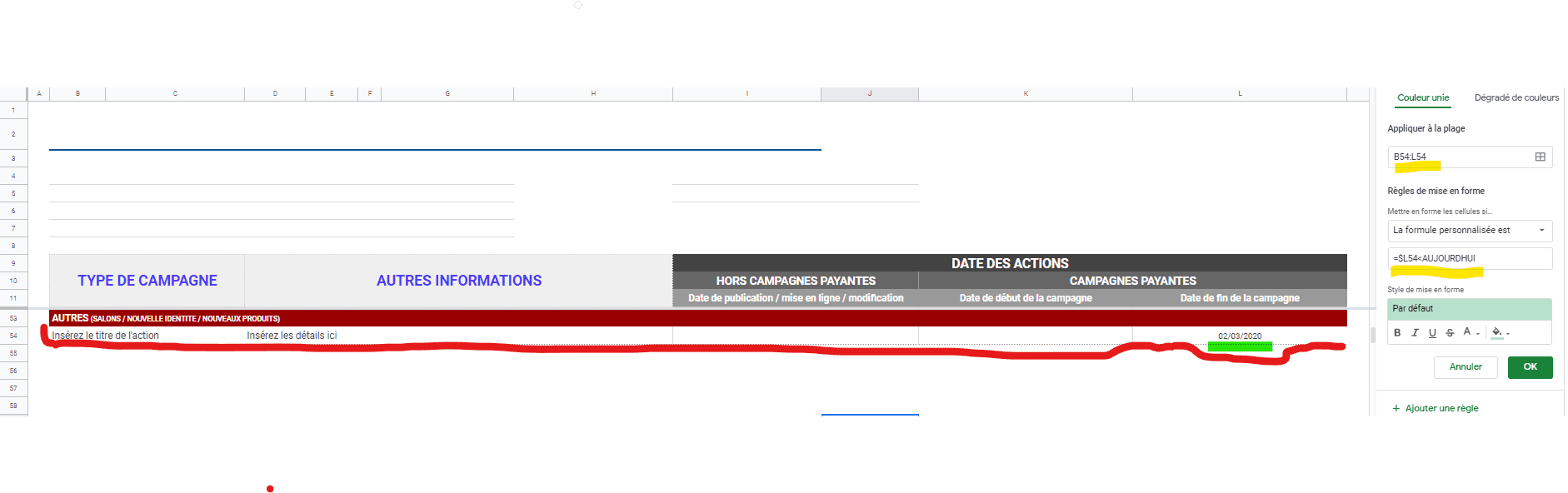
I’m sending you a screenshot for better understanding:
- Green = Cell containing the value
- Yellow = Formula I tried to use.
- Red = Cells that should turn gray based on the green cell.
Thank you in advance.
Configuration: Windows / Chrome 80.0.3987.132
I want to set up an action plan for ongoing/completed tasks in my company.
To facilitate reading, I would like the entire line to turn gray once the task is finished (Example: Action completed on 10/03/2020 while we are on 11/03/2020).
However, after trying several times I am encountering several problems:
1. The formatting does not apply to all formulas.
2. The formula does not adapt to the chosen cell if I drag it down.
3. When I insert a row below, the entire format of the row does not replicate. Do you have a trick?
The purpose of this document is to hand it over to my salespeople so they can fill it out as easily as possible. Therefore, everything should be optimized when they add a row.
I’m sending you a screenshot for better understanding:
- Green = Cell containing the value
- Yellow = Formula I tried to use.
- Red = Cells that should turn gray based on the green cell.
Thank you in advance.
Configuration: Windows / Chrome 80.0.3987.132
Related links:
- conditional formatting with 3 conditions
- Conditional formatting with multiple conditions
- color a cell based on the value of another cell
- Conditional formatting for deadlines Google Sheets
- Google Sheets: Conditional Formatting for Expired Dates.
- Conditional formatting: Highest and lowest value by row
4 answers
-
Hello
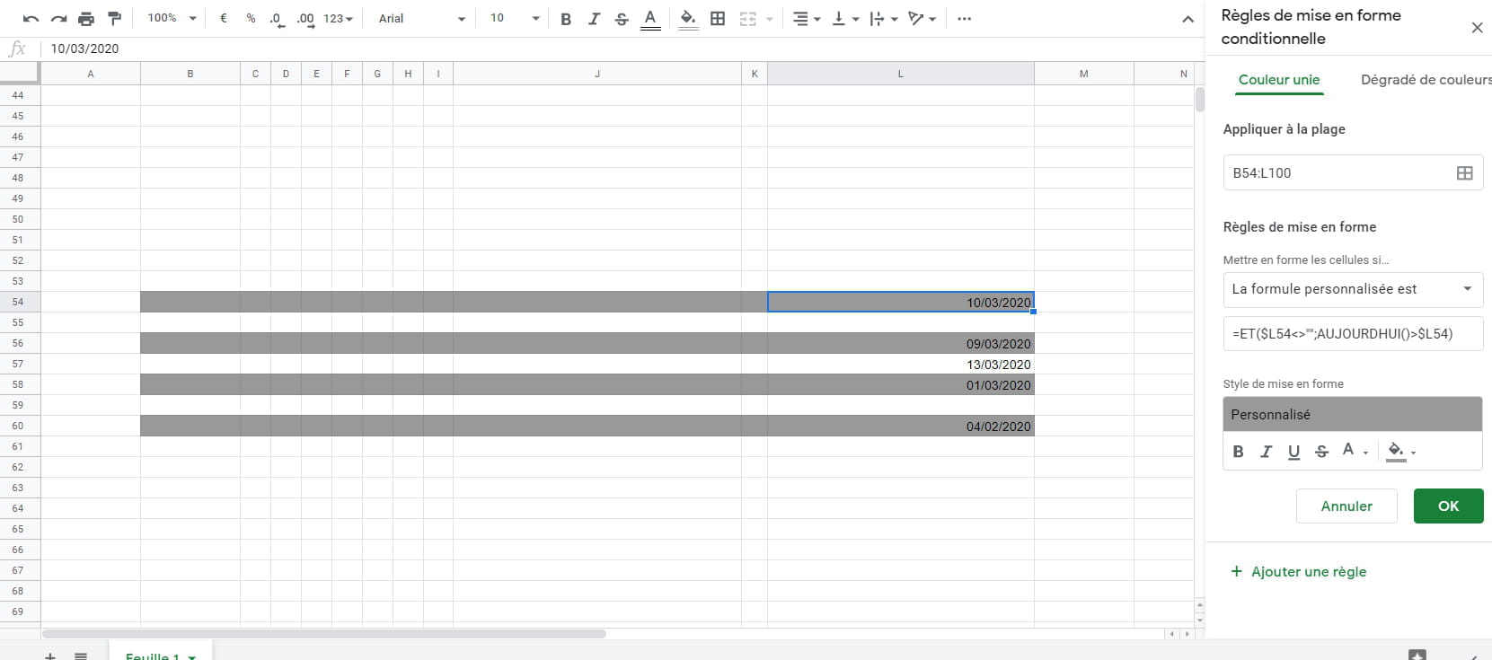
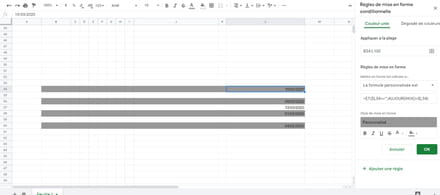
The best way is to apply the conditional formatting over a predefined area and indicate in the formula that the cell in column L must necessarily contain a date for it to work; otherwise, it remains blank.
Select the entire area (e.g., B54:L100) and use this formula:
=AND($L54<>"";TODAY()>$L54)
Thus, as soon as a date earlier than today’s date is entered, the row will be colored gray.
Best regards -
Hello,
So a click on resolved to confirm
Best regards. -
Hello,
I would like to ask you an additional question.
Can I also add column IJ 54 to the formula so that when one of my colleagues types a past upload date, the entire row turns gray as well?
Thank you in advance.
Kind regards. -
Hello,
Is IJ54 very far??? I assume these are I54 and J54.
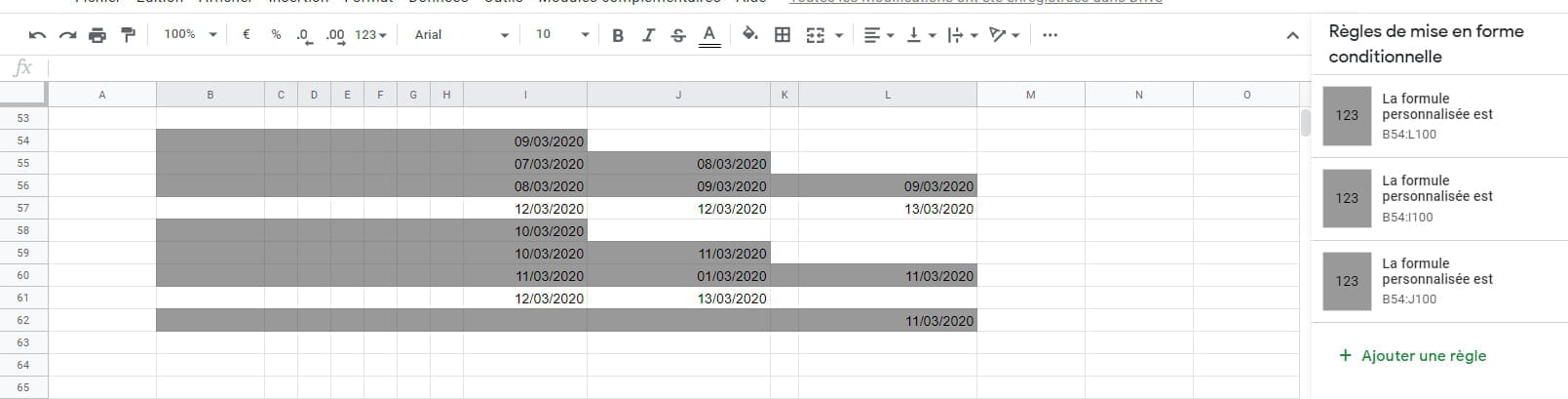
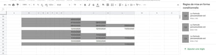
To avoid confusion, I recommend a gradual advancement of the gray area with a gradient of gray or not; therefore, using two conditional formatting rules in addition
1 / select the area (B54:I100 to use the same example)
The formula: =AND($I54<>"", TODAY()>$I54)
2 / select the area (B54:J100)
the formula: =AND($J54<>"", TODAY()>$J54)
If this is not what you want, please explain your request a bit better.
Best regards.