Conditional formatting that changes for each row
Solved
AnthonyKimo
Posted messages
10
Registration date
Status
Member
Last intervention
-
PapyLuc51 Posted messages 4567 Registration date Status Member Last intervention -
PapyLuc51 Posted messages 4567 Registration date Status Member Last intervention -
Hello everyone.
I’m visiting this forum, I’ll admit it as a last resort, after trying many attempts to achieve what I was trying to set up...But I must come to terms with it, either my knowledge is too limited or Excel cannot do it.
I have a table, where the columns are:
The name of a place
A total turnover figure
3 columns with lower turnover figures, normal turnover figures and higher turnover figures
Then 12 columns representing the 12 months of the year.
In each row the name of the place.

I’m attaching an image to make it easier to decipher.
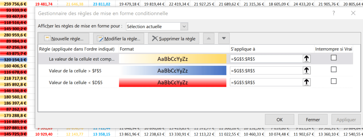
My goal is to reproduce the conditional formatting of row 5 across the entire table!
Unfortunately my conditional formatting only applies to that row. When I drag it with the fill handle across the entire table I don’t get the desired result.
That is, for row 5 I want
In red the figures below the insufficent CA (Column D)
In yellow the figures between the CA column D and the CA upper column F
In blue the figures above the sufficient CA column F
But I want the same thing for row 6 relative to the data of row 6, Row 7, 8, etc.

When I copy the conditional formatting, the whole table then references the value of row 5.
I tried in the conditional formatting rules to remove the $ in the reference value, but the same, some values end up red even though they should be blue, I changed the order of the rules... Nothing works.
So I’m coming to this forum to ask for a bit of help :)
Or a few tips that could help me solve this puzzle, please.
Thank you in advance
Anthony
I’m visiting this forum, I’ll admit it as a last resort, after trying many attempts to achieve what I was trying to set up...But I must come to terms with it, either my knowledge is too limited or Excel cannot do it.
I have a table, where the columns are:
The name of a place
A total turnover figure
3 columns with lower turnover figures, normal turnover figures and higher turnover figures
Then 12 columns representing the 12 months of the year.
In each row the name of the place.
I’m attaching an image to make it easier to decipher.
My goal is to reproduce the conditional formatting of row 5 across the entire table!
Unfortunately my conditional formatting only applies to that row. When I drag it with the fill handle across the entire table I don’t get the desired result.
That is, for row 5 I want
In red the figures below the insufficent CA (Column D)
In yellow the figures between the CA column D and the CA upper column F
In blue the figures above the sufficient CA column F
But I want the same thing for row 6 relative to the data of row 6, Row 7, 8, etc.
When I copy the conditional formatting, the whole table then references the value of row 5.
I tried in the conditional formatting rules to remove the $ in the reference value, but the same, some values end up red even though they should be blue, I changed the order of the rules... Nothing works.
So I’m coming to this forum to ask for a bit of help :)
Or a few tips that could help me solve this puzzle, please.
Thank you in advance
Anthony