Excel: If names are identical, then sum the associated numbers. Solved

Question

Hello,  here is the situation: it involves grouping cells by names and summing the tonnages associated with these names in the same row.  the goal is to know the quantities collected in several different containers (which are therefore separated in the table) but are located in the same place.  the problem is that I don’t want to say: “if column A = so-and-so name, add the numbers in column B.” No. I want to be able to ask: “if names in column A are identical (without specifying a particular name), then add the numbers from column B.” I do not want to specify a particular name in column A because there are several different names that need to be grouped. I just want to ask to group the names that are the same and sum the corresponding numbers.  example column A:  3 MOUSQUETAIRES-HERBLAY ATAC-HOUILLES ATAC-HOUILLES BABOU-LES MUREAUX BABOU-LES MUREAUX BOIS D'ARCY - Leclerc BOIS D'ARCY - Leclerc BOIS D'ARCY - Leclerc BOIS D'ARCY - Leclerc BOIS D'ARCY - Leclerc BOIS D'ARCY - Leclerc BUCHELAY - Auchan BUCHELAY - Auchan BUCHELAY - Auchan BUCHELAY - Auchan   I’m not sure if I was clear. Thank you in advance.  JB  Configuration: Windows 7 / Chrome 43.0.2357.130

Excel-worker · Accepted Answer

Hello,  I am taking Eriiic's solution with an example; maybe this will clarify things for you.  File: https://www.cjoint.com/c/EGgmQgR1jT3  Best regards, Excel-Worker -- "Our greatest glory is not in never falling, but in rising every time we fall." Confucius

eriiic · Answer

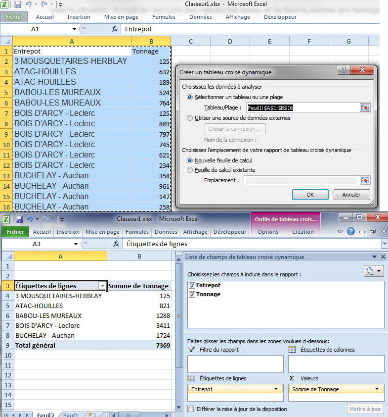
Hello,  Insert a Pivot Table (TCD): http://www.mdf-xlpages.com/modules/publisher/item.php?itemid=109 eric  -- By continuously trying, we eventually succeed. So the more it fails, the more chances we have that it will work. (the Shadoks) In addition to the thank you (yes, it’s done!!!), remember to mark it as resolved. Thank you

Vaucluse · Answer

Hello  it's not easy to understand your problem try this, (whether the list is sorted by location name or not) list of names in A starting from A1 list of weights in B starting from B2  in C2 the formula:  =IF(COUNTIF($A$1:A1,A2)=0,SUMIF(A:A,A2,B:B),"") this formula will give you the cumulative amount corresponding to the name in A2 only on the row where the name appears for the first time in the list, the others remaining without display (if you properly respect the $ of the first A1)  to have the total next to the last, on a table of 1000 rows in A2: =IF(COUNTIF(A23:$A$1000,A2)=0,SUMIF(A:A,A2,B:B)  to have an evolving sum each time you find the name: =SUMIF($A$2,A2,A2,$B$2:B2)  etc  best regards  -- To err is human, to persist is diabolical

jibejou · Answer

OK, thanks everyone. I struggled a bit but finally succeeded.  In fact, it's important to know that the designations must be sorted, so the same designations should be listed one after the other in the source table (which wasn’t obvious in my case). And if there are empty cells in the values (which was my case), you need to modify the value function once the dynamic table is created to request the "sum" function instead of "count." To do this: small menu arrow: "value field settings." Again, it would be clearer with images, but perfection is the enemy of good, isn't it? ;)  Thanks again, everyone! JB

Excel: If names are identical, then sum the associated numbers.

4 réponses

Texture issues in enshrouded

Old lullaby

Unable to connect to freebox os

Edit ad on leboncoin for free

Freebox wifi password

Computer tower that won't turn on

Blocked: are my messages still being delivered?

Video intercom inspector

Your computer can't use another display.

Fransat decoder stuck